Protein-level analysis: reproducing Karayel et al. (2020)
This notebook demonstrates a protein-level analysis workflow using ProteoPy, reproducing selected results from Karayel et al. (2020):
Karayel Ö, Xu P, Bludau I, Velan Bhoopalan S, Yao Y, Ana Rita FC, Santos A, Schulman BA, Alpi AF, Weiss MJ, and Mann M. Integrative proteomics reveals principles of dynamic phosphosignaling networks in human erythropoiesis. Molecular Systems Biology, 16(12):MSB20209813, 2020. doi:10.15252/msb.20209813
The authors profiled the proteome across five stages of in vitro erythropoiesis from CD34⁺ HSPCs — progenitors, proerythroblasts and early basophilic erythroblasts (ProE&EBaso), late basophilic erythroblasts (LBaso), polychromatic erythroblasts (Poly), and orthochromatic erythroblasts (Ortho) — using DIA-based mass spectrometry with four biological replicates per stage. They quantified ~7,400 proteins, demonstrating high reproducibility within stages, stage-specific proteome remodeling driven by drastic transitions at the progenitor-to-ProE/EBaso and Poly-to-Ortho boundaries, and hierarchical clustering revealing six distinct co-expression profiles across differentiation.
Here, we reproduce the core protein-level analysis including quality control, normalization, dimensionality reduction (Figures 1C–D, 2A), differential abundance testing (Figure 2D), and hierarchical clustering of expression profiles (Figure 2B).
Setup
[1]:
# Jupyter autoreload for development
%load_ext autoreload
%autoreload 2
[2]:
import os
import random
from pathlib import Path
import numpy as np
import pandas as pd
import anndata as ad
import scanpy as sc
import matplotlib.pyplot as plt

import proteopy as pr  # Convention: import proteopy as pr

random.seed(42)

cwd = Path('.').resolve()
root = cwd.parents[1]
os.chdir(root)
/home/ifichtner/miniforge3/envs/proteopy-usage2/lib/python3.10/site-packages/tqdm/auto.py:21: TqdmWarning: IProgress not found. Please update jupyter and ipywidgets. See https://ipywidgets.readthedocs.io/en/stable/user_install.html
  from .autonotebook import tqdm as notebook_tqdm
Reading in the data
The Karayel et al. (2020) dataset contains protein-level DIA-MS intensities from five erythroid differentiation stages of CD34⁺ HSPCs. ProteoPy provides a built-in download function (pr.download.karayel_2020()) that fetches the dataset from the PRIDE archive (PXD017276), processes it, and saves it as three separate files:
Intensities — long-format table with columns
sample_id,protein_id, andintensity(one row per measurement)Sample annotation — maps each
sample_idto itscell_typeandreplicateProtein annotation — maps each
protein_idto itsgene_id
This separation into three files mirrors a common data delivery format in proteomics. The files are then read into an AnnData object using pr.read.long().
[4]:
intensities_path = "data/karayel-2020_ms-proteomics_human-erythropoiesis_intensities.tsv"
sample_annotation_path = "data/karayel-2020_ms-proteomics_human-erythropoiesis_sample-annotation.tsv"
var_annotation_path = "data/karayel-2020_ms-proteomics_human-erythropoiesis_protein-annotation.tsv"

pr.download.karayel_2020(
    intensities_path=intensities_path,
    sample_annotation_path=sample_annotation_path,
    var_annotation_path=var_annotation_path,
    force=True,  # Overwrite files if already exist
)
A quick look at the first rows of each file confirms the expected structure:
[5]:
!head -n5 {intensities_path}
sample_id       protein_id      intensity
LBaso_rep1      A0A024QZ33;Q9H0G5       15084.2626953125
LBaso_rep2      A0A024QZ33;Q9H0G5       15442.2646484375
LBaso_rep3      A0A024QZ33;Q9H0G5       13992.021484375
LBaso_rep4      A0A024QZ33;Q9H0G5       18426.5390625
[6]:
!head -n5 {sample_annotation_path}
sample_id       cell_type       replicate
LBaso_rep1      LBaso   rep1
LBaso_rep2      LBaso   rep2
LBaso_rep3      LBaso   rep3
LBaso_rep4      LBaso   rep4
[7]:
!head -n5 {var_annotation_path}
protein_id      gene_name
A0A024QZ33;Q9H0G5       NSRP1
A0A024QZB8;A0A0A0MRC7;A0A0D9SFH9;A0A1B0GV71;A0A1B0GW34;A0A1B0GWD3;H3BR00;Q13286;Q13286-2;Q13286-3;Q13286-4;Q13286-5;Q9UBD8      CLN3;CLN3;CLN3;CLN3;CLN3;;CLN3;CLN3;CLN3;CLN3;CLN3;CLN3;CLN3
A0A024R0Y4;O75478       TADA2A
A0A024R216;Q9Y3E1       HDGFRP3;HDGFL3
With the three files on disk, pr.read.long() reads the long-format intensities, pivots them into a dense matrix, and merges the sample and protein annotations into a single AnnData object. Setting fill_na=0 replaces any missing intensity values with zero.
[ ]:
adata = pr.read.long(
    intensities=intensities_path,
    level='protein',
    sample_annotation=sample_annotation_path,
    var_annotation=var_annotation_path,
    fill_na=0,
)

adata
[8]:
# Validate that the loaded data conforms to proteodata format
from proteopy.utils.anndata import check_proteodata

check_proteodata(adata)
[8]:
(True, 'protein')
[9]:
# Store color scheme in .uns for consistent plotting across the tutorial
adata.uns['colors_cell_type'] = {
    "LBaso": "#D91C5C",
    "Ortho": "#F6922F",
    "Poly": "#262261",
    "ProE&EBaso": "#1B75BB",
    "Progenitor": "#D6DE3B",
}

# Define haemoglobin proteins for highlighting (marker proteins in erythropoiesis)
haemoglobin = {
    'F8W6P5': 'HBB1',
    'P69905': 'HBA1',
    'P02100': 'HBE1',
    'A0A2R8Y7X9;P69891': 'HBG1',
}

# Store differentiation order once for consistent plotting
adata.uns['diff_order'] = ['Progenitor', 'ProE&EBaso', 'LBaso', 'Poly', 'Ortho']
Quality control and preprocessing
The dataset contains 20 samples (5 stages x 4 replicates) and ~7,750 protein groups. We apply standard QC steps: contaminant removal, completeness-based filtering, and visual inspection of abundance distributions and reproducibility (related to Figure 1C–D).
Abundance rank plot
[ ]:
# Haemoglobin proteins are highlighted
pr.pl.abundance_rank(
    adata,
    color='cell_type',
    log_transform=10,
    zero_to_na=True,            # Treat zeros as missing values
    color_scheme=adata.uns["colors_cell_type"],
    summary_method='median',
    highlight_vars=list(haemoglobin.keys()),
    var_labels_key='gene_id', # Use gene names instead of protein IDs for labels
    )
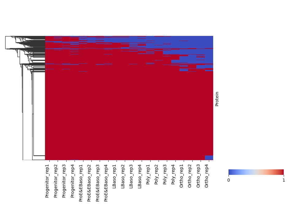
Binary detection heatmap
[ ]:
# Binary heatmap: proteins above threshold are encoded as 1 (present), otherwise 0
pr.pl.binary_heatmap(
adata,
threshold=0,
order_by='cell_type',
order=adata.uns['diff_order'],
col_cluster=False,
row_cluster=True,
figsize=(10, 6),
)
/opt/homebrew/Caskroom/miniforge/base/envs/proteopy1/lib/python3.11/site-packages/seaborn/matrix.py:560: UserWarning: Clustering large matrix with scipy. Installing `fastcluster` may give better performance.
  warnings.warn(msg)
Contaminant removal
[12]:
# Download contaminant FASTA (sources: 'frankenfield2022', 'gpm-crap')
contaminants_path = pr.download.contaminants(source='frankenfield2022')

# Remove proteins matching contaminant sequences
pr.pp.remove_contaminants(
    adata,
    contaminant_path=contaminants_path,
    inplace=True,  # Modify adata directly (default behavior)
    )
Removed 12 contaminating proteins.
/Users/leventetn/Documents/Proteopy/proteopy/proteopy/download/contaminants.py:140: UserWarning: File already exists at data/contaminants_frankenfield2022_2026-02-28.fasta. Use force=True to overwrite.
  warnings.warn(
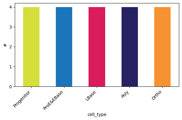
By study design, the dataset includes 5 differentiation stages with 4 biological replicates each:
[13]:
pr.pl.n_samples_per_category(
        adata,
        category_key='cell_type',
        color_scheme=adata.uns['colors_cell_type'],
        order=adata.uns['diff_order'],
        )
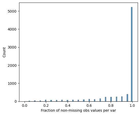
Completeness filtering
Proteins are retained if they are detected in all replicates of at least one differentiation stage:
[14]:
# Visualize protein completeness before filtering
pr.pl.completeness_per_var(adata, zero_to_na=True)
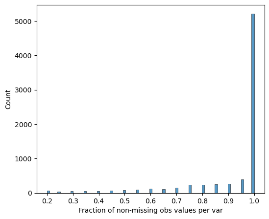
[15]:
# Require 100% completeness within at least one cell type (group_by='cell_type')
# This keeps proteins that are consistently measured in at least one cell type.
pr.pp.filter_var_completeness(
    adata,
    min_fraction=1,
    group_by='cell_type',
    zero_to_na=True,
    )
277 var removed
[16]:
# Verify completeness after filtering
pr.pl.completeness_per_var(adata, zero_to_na=True)
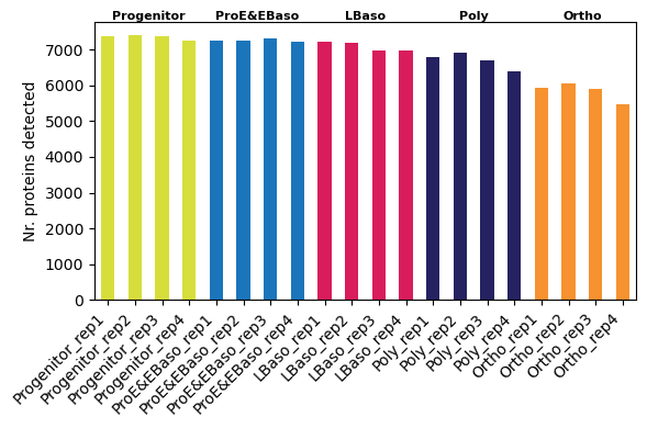
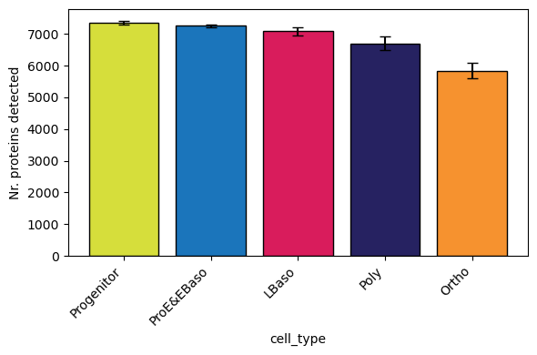
Proteins per sample (reproduces Figure 1C)
Consistent with Karayel et al., the number of quantified proteins decreases along the differentiation trajectory:
[17]:
# Per-sample protein counts (individual bars)
pr.pl.n_proteins_per_sample(
    adata,
    zero_to_na=True,
    order_by='cell_type',
    order=adata.uns['diff_order'],
    color_scheme=adata.uns['colors_cell_type'],
    xlabel_rotation=45,
    )
[18]:
# Grouped by cell type (boxplot per group) - reproduces Figure 1C from Karayel et al.
pr.pl.n_proteins_per_sample(
    adata,
    zero_to_na=True,
    group_by='cell_type',  # Aggregate samples into boxplots per group
    order=adata.uns['diff_order'],
    color_scheme=adata.uns['colors_cell_type'],
    xlabel_rotation=45,
    )
[19]:
# Remove samples with fewer than 6000 detected proteins
pr.pp.filter_samples(adata, min_count=6000)
0 obs removed
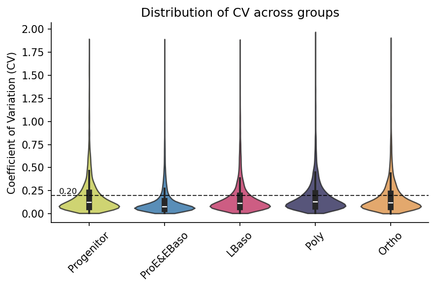
Coefficient of variation
Intra-group CVs confirm high technical reproducibility across replicates:
[20]:
# Calculate CV per protein within each cell type (stored in adata.var)
pr.pp.calculate_cv(adata, group_by='cell_type', min_samples=3)
[21]:
# Visualize CV distribution per group (hline shows typical 20% CV threshold)
pr.pl.cv_by_group(
    adata,
    group_by='cell_type',
    color_scheme=adata.uns["colors_cell_type"],
    figsize=(6, 4),
    xlabel_rotation=45,
    order=adata.uns['diff_order'],
    hline=0.2,  # Reference line at 20% CV
    )
Using existing CV data from adata.varm['cv_by_cell_type_X'].
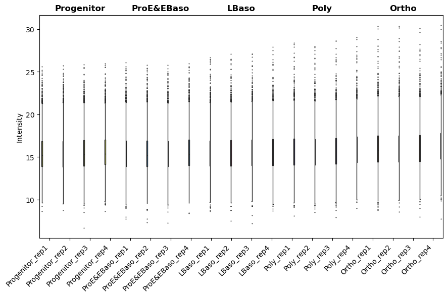
Data transformation
Log2 transformation, median normalization, and down-shift imputation of missing values.
[22]:
# Convert zeros to NaN (missing values) and log2 transform
# Note: Save raw data in `layers` and then modigy adata.X directly
adata.layers['raw'] = adata.X.copy()
adata.X[adata.X == 0] = np.nan
adata.X = np.log2(adata.X)
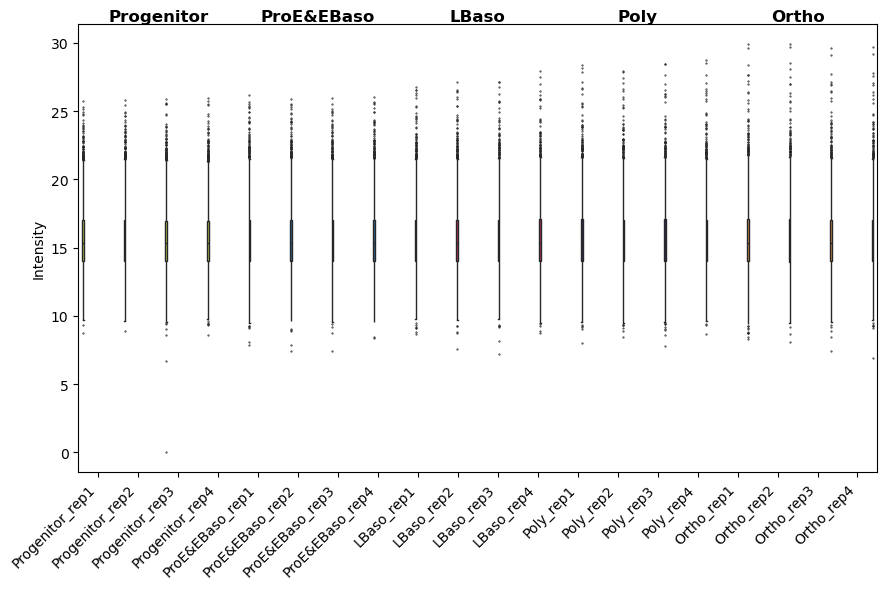
Median normalization
[23]:
# Visualize intensity distributions between samples first
pr.pl.intensity_box_per_sample(
    adata,
    order_by='cell_type',
    order=adata.uns['diff_order'],
    zero_to_na=True,
    color_scheme=adata.uns['colors_cell_type'],
    xlabel_rotation=45,
    figsize=(9, 6),
    )
[23]:
<Axes: ylabel='Intensity'>
[24]:
# Apply median normalization (target='median' uses the median of sample-level medians as a scaling factor.)
pr.pp.normalize_median(
    adata,
    target='median',
    log_space=True, # log_space=True indicates data is already log-transformed
    )
[25]:
# After normalization: distributions should be aligned
pr.pl.intensity_box_per_sample(
    adata,
    order_by='cell_type',
    order=adata.uns['diff_order'],
    zero_to_na=True,
    color_scheme=adata.uns['colors_cell_type'],
    xlabel_rotation=45,
    figsize=(9, 6),
    )
[25]:
<Axes: ylabel='Intensity'>
Down-shift imputation
[26]:
# Impute missing values using down-shift method
# downshift: How many std devs below mean to center imputed values
# width: Width of the imputation distribution (std devs)
pr.pp.impute_downshift(
    adata,
    downshift=1.8,
    width=0.3,
    zero_to_nan=True,
    random_state=123,  # For reproducibility
    )
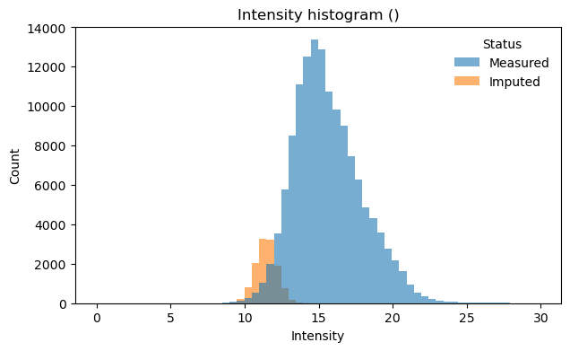
[27]:
# Nr of measured and imputed values
mask = np.asarray(adata.layers["imputation_mask_X"], dtype=bool)
measured_n = int((~mask).sum())
imputed_n = int(mask.sum())
print(f"Measured: {measured_n:,} values ({100*measured_n/(measured_n+imputed_n):.1f}%)")
print(f"Imputed: {imputed_n:,} values ({100*imputed_n/(measured_n+imputed_n):.1f}%)")
Measured: 136,962 values (91.7%)
Imputed: 12,418 values (8.3%)
[28]:
# Visualize intensity distribution with imputed values highlighted
# Combined histogram across all samples
pr.pl.intensity_hist(
adata,
color_imputed=True, # Color imputed vs measured values differently
density=False,
)
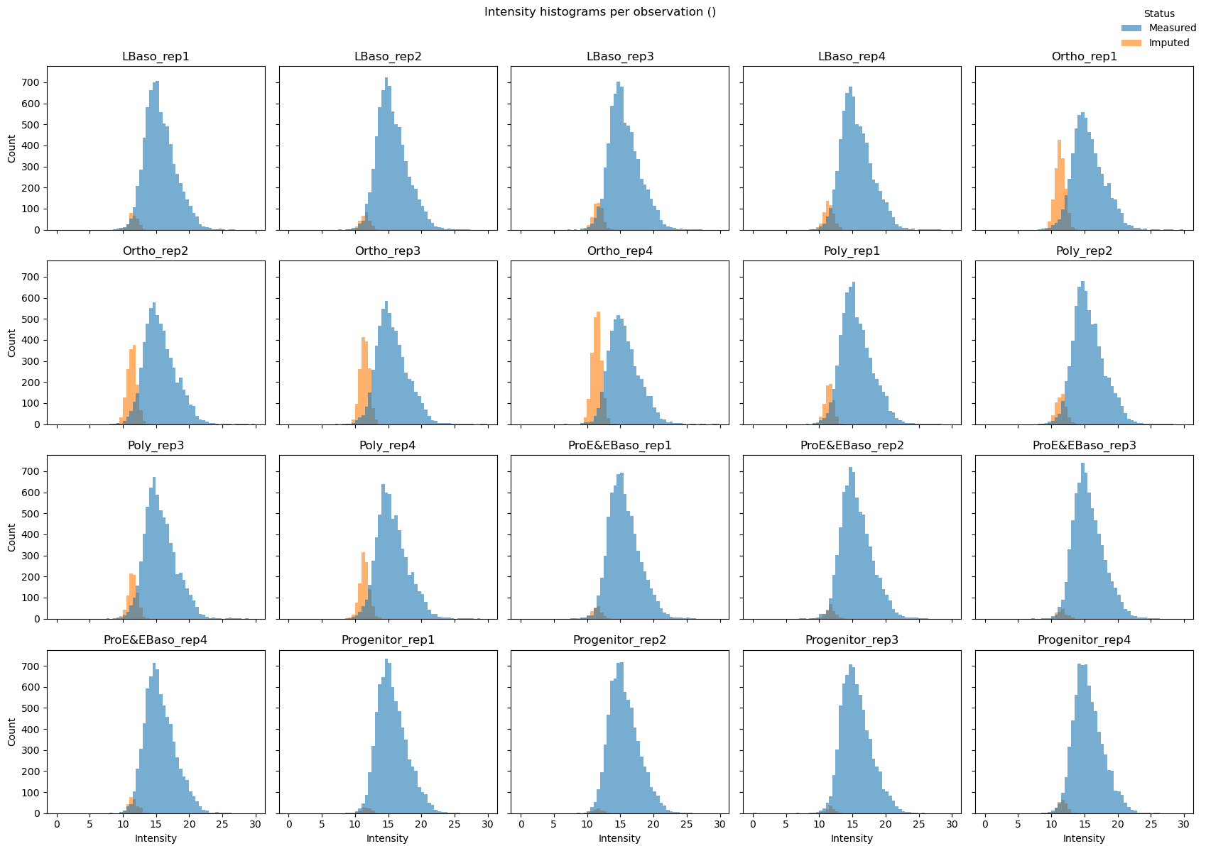
# Per-sample histograms (small multiples)
pr.pl.intensity_hist(
adata,
color_imputed=True,
per_obs=True, # One subplot per sample
ncols=5,
legend_loc="upper right",
density=False,
figsize=(17, 12),
)
Exploratory analysis
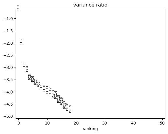
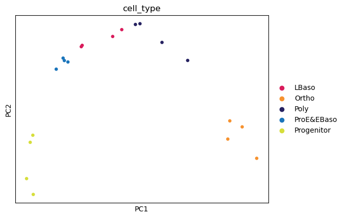
PCA (reproduces Figure 2A)
The five differentiation stages separate along the first two principal components, with PC1 (43.3% variance) resolving the main differentiation axis from progenitors to orthochromatic erythroblasts.
[29]:
# PCA using scanpy (ProteoPy AnnData is fully compatible)
sc.tl.pca(adata)
sc.pl.pca_variance_ratio(adata, n_pcs=50, log=True)
sc.pl.pca(
    adata,
    color='cell_type',
    dimensions=(0, 1),
    ncols=2,
    size=90,
    palette=adata.uns['colors_cell_type'],
    )
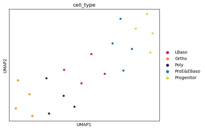
UMAP
[30]:
# UMAP for non-linear dimensionality reduction
sc.pp.neighbors(adata, n_neighbors=6)
sc.tl.umap(adata)
sc.pl.umap(
    adata,
    color='cell_type',
    size=100,
    palette=adata.uns['colors_cell_type'],
    )
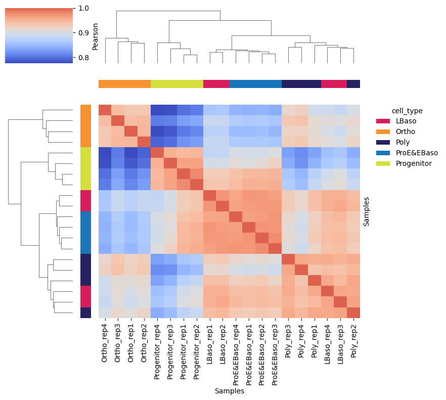
Sample correlation matrix (reproduces Figure 1D)
High intra-stage Pearson correlations (r > 0.95) and clear inter-stage structure confirm biological reproducibility and stage-specific proteome remodeling.
[31]:
# Clustered sample correlation heatmap with cell type annotation on margins
pr.pl.sample_correlation_matrix(
    adata,
    method="pearson",
    margin_color="cell_type",  # Color bar annotation
    color_scheme=adata.uns["colors_cell_type"],
    xticklabels=True,
    figsize=(9, 8),
    linkage_method='average',
    )
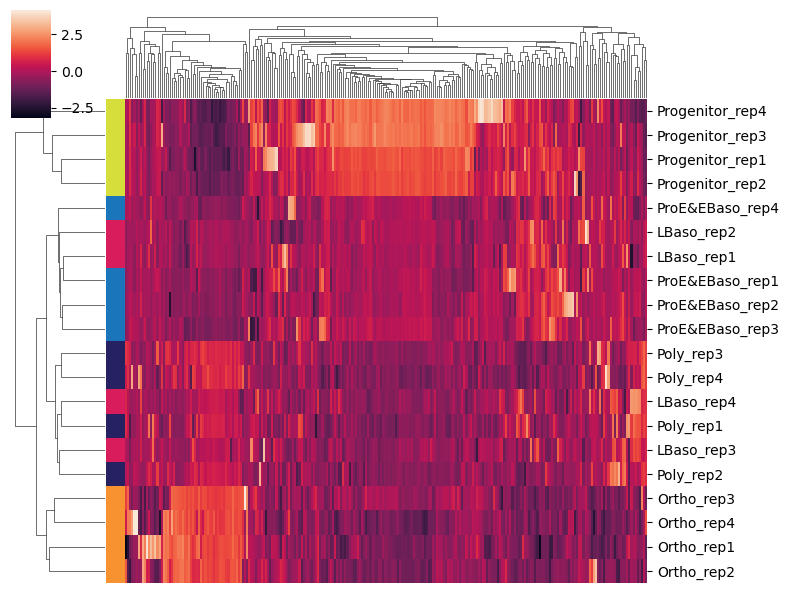
Highly variable proteins
[32]:
# Use scanpy's HVG detection (marks top 250 most variable proteins in adata.var)
sc.pp.highly_variable_genes(
    adata,
    n_top_genes=250,
    inplace=True,
    )
[33]:
# Subset to highly variable proteins and plot clustered heatmap
adata_hvg = adata[:, adata.var['highly_variable']].copy()

sc.pl.clustermap(
    adata_hvg,
    obs_keys='cell_type',
    z_score=1,          # Z-score normalize per protein (row)
    figsize=(8, 6),
    dendrogram_ratio=0.15,
    show=True,
    xticklabels=False,  # Too many proteins for labels
    )
Differential abundance analysis
One-vs-rest t-tests identify stage-specific proteins. Karayel et al. reported 4,316 differentially abundant proteins (ANOVA, FDR < 0.01), with the most drastic changes at the progenitor-to-ProE/EBaso and Poly-to-Ortho transitions (Figure 2C–D).
[34]:
# One-vs-rest t-tests for each cell type (results stored in adata.varm)
pr.tl.differential_abundance(
    adata,
    method="ttest_two_sample",
    group_by='cell_type',
    setup={},               # Empty = one-vs-rest for all groups
    multitest_correction='bh',  # Benjamini-Hochberg FDR correction
    alpha=0.05,
    space='log',            # Data is in log space
    )
Saved test results in .varm['ttest_two_sample;cell_type;LBaso_vs_rest']
Saved test results in .varm['ttest_two_sample;cell_type;Ortho_vs_rest']
Saved test results in .varm['ttest_two_sample;cell_type;Progenitor_vs_rest']
Saved test results in .varm['ttest_two_sample;cell_type;ProE_EBaso_vs_rest']
Saved test results in .varm['ttest_two_sample;cell_type;Poly_vs_rest']
Test results are stored in adata.varm and can be retrieved as DataFrames:
[35]:
# List all stored test results
pr.get.tests(adata)
[35]:
| key | key_group | test_type | group_by | design | design_label | design_mode | layer | |
|---|---|---|---|---|---|---|---|---|
| 0 | ttest_two_sample;cell_type;LBaso_vs_rest | ttest_two_sample;cell_type;one_vs_rest | ttest_two_sample | cell_type | LBaso_vs_rest | LBaso vs rest | one_vs_rest | None |
| 1 | ttest_two_sample;cell_type;Ortho_vs_rest | ttest_two_sample;cell_type;one_vs_rest | ttest_two_sample | cell_type | Ortho_vs_rest | Ortho vs rest | one_vs_rest | None |
| 2 | ttest_two_sample;cell_type;Progenitor_vs_rest | ttest_two_sample;cell_type;one_vs_rest | ttest_two_sample | cell_type | Progenitor_vs_rest | Progenitor vs rest | one_vs_rest | None |
| 3 | ttest_two_sample;cell_type;ProE_EBaso_vs_rest | ttest_two_sample;cell_type;one_vs_rest | ttest_two_sample | cell_type | ProE_EBaso_vs_rest | ProE EBaso vs rest | one_vs_rest | None |
| 4 | ttest_two_sample;cell_type;Poly_vs_rest | ttest_two_sample;cell_type;one_vs_rest | ttest_two_sample | cell_type | Poly_vs_rest | Poly vs rest | one_vs_rest | None |
[36]:
# Get significant proteins across all one-vs-rest tests (|logFC| >= 1, p_adj < 0.05)
pr.get.differential_abundance_df(
    adata,
    key_group='ttest_two_sample;cell_type;one_vs_rest',  # All one-vs-rest tests
    min_logfc=1,        # Minimum absolute log2 fold change
    max_pval=0.05,      # Maximum adjusted p-value
    sort_by='pval_adj', # Sort by adjusted p-value
    )
[36]:
| var_id | test_type | group_by | design | mean1 | mean2 | logfc | tstat | pval | pval_adj | is_diff_abundant | |
|---|---|---|---|---|---|---|---|---|---|---|---|
| 0 | Q8IXW5;Q8IXW5-2 | ttest_two_sample | cell_type | Ortho_vs_rest | 21.060375 | 12.935327 | 8.125048 | 23.517326 | 5.778442e-15 | 3.114776e-11 | True |
| 1 | E7ESC6 | ttest_two_sample | cell_type | Ortho_vs_rest | 19.692222 | 16.984114 | 2.708108 | 16.811764 | 1.885384e-12 | 7.040966e-10 | True |
| 2 | Q8TB52 | ttest_two_sample | cell_type | Ortho_vs_rest | 16.234364 | 13.902348 | 2.332016 | 15.007092 | 1.278869e-11 | 2.449197e-09 | True |
| 3 | Q7Z333;Q7Z333-4 | ttest_two_sample | cell_type | Ortho_vs_rest | 16.963578 | 15.899757 | 1.063821 | 14.861999 | 1.504470e-11 | 2.613229e-09 | True |
| 4 | O43516;O43516-2;O43516-3;O43516-4 | ttest_two_sample | cell_type | Progenitor_vs_rest | 15.411008 | 11.522910 | 3.888098 | 16.436716 | 2.763870e-12 | 1.104769e-08 | True |
| ... | ... | ... | ... | ... | ... | ... | ... | ... | ... | ... | ... |
| 956 | Q6UW63 | ttest_two_sample | cell_type | Progenitor_vs_rest | 15.015388 | 13.067117 | 1.948270 | 2.778024 | 1.240691e-02 | 4.915014e-02 | True |
| 957 | Q9UPY3 | ttest_two_sample | cell_type | Progenitor_vs_rest | 13.912874 | 12.656495 | 1.256379 | 2.777509 | 1.242059e-02 | 4.916237e-02 | True |
| 958 | J9JIC5;Q9HAS0 | ttest_two_sample | cell_type | Progenitor_vs_rest | 13.641169 | 12.517267 | 1.123901 | 2.774577 | 1.249870e-02 | 4.931474e-02 | True |
| 959 | H0YH69;Q9HBU6 | ttest_two_sample | cell_type | Progenitor_vs_rest | 13.984629 | 12.503137 | 1.481492 | 2.771020 | 1.259412e-02 | 4.953421e-02 | True |
| 960 | A0A075B6E4;A0A0A6YYI5;G5E9M7;G5E9M9;Q14135;Q14... | ttest_two_sample | cell_type | Progenitor_vs_rest | 12.950283 | 11.872185 | 1.078098 | 2.766072 | 1.272799e-02 | 4.990309e-02 | True |
961 rows × 11 columns
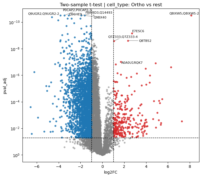
Volcano plot (related to Figure 2D)
[37]:
# Volcano plot for Ortho vs rest comparison
pr.pl.volcano_plot(
    adata,
    varm_slot='ttest_two_sample;cell_type;Ortho_vs_rest',
    fc_thresh=1,        # Fold change threshold lines
    pval_thresh=0.05,   # P-value threshold line
    xlabel='log2FC',
    ylabel_logscale=True,
    top_labels=5,       # Label top 5 most significant
    figsize=(8, 7),
    )
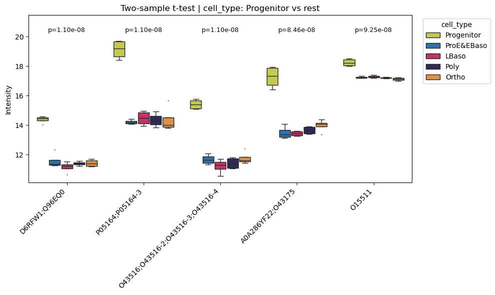
Top differentially abundant proteins
[38]:
# Box plots for top 5 differentially abundant proteins (Progenitor vs rest)
pr.pl.differential_abundance_box(
    adata,
    varm_slot='ttest_two_sample;cell_type;Progenitor_vs_rest',
    top_n=5,
    color_scheme=adata.uns['colors_cell_type'],
    order=adata.uns['diff_order'],
    )
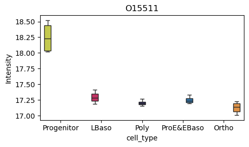
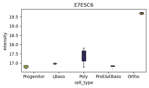
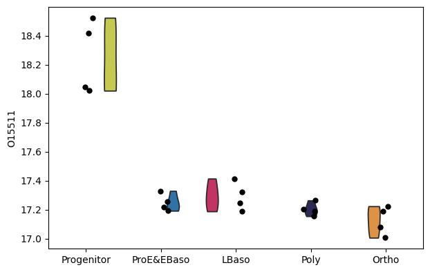
[39]:
# Box plot for a specific protein of interest
pr.pl.box(
    adata,
    keys=['O15511', 'E7ESC6'],
    group_by='cell_type',
    order=['Progenitor', 'LBaso', 'Poly', 'ProE&EBaso', 'Ortho'],
    color_scheme=adata.uns['colors_cell_type'],
    figsize=(5,3),
    )
[40]:
# Alternative: use scanpy's violin plot
sc.pl.violin(
    adata,
    keys=['O15511'],
    groupby='cell_type',
    order=adata.uns['diff_order'],
    size=6,
    xlabel=None,
    )
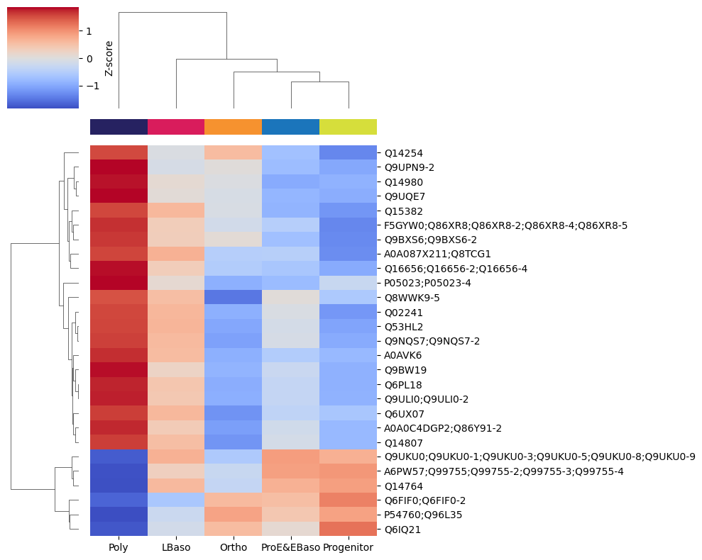
Hierarchical clustering of expression profiles (reproduces Figure 2B)
Karayel et al. performed hierarchical clustering of differentially abundant proteins, revealing six distinct temporal co-expression profiles across the five differentiation stages. We reproduce this analysis using ProteoPy’s hierarchical clustering tools.
[41]:
# Get differentially abundant proteins for Poly vs rest
df = pr.get.differential_abundance_df(
    adata,
    keys='ttest_two_sample;cell_type;Poly_vs_rest',
    )
diff_prots = df[df['pval_adj'] <= 0.05]

# Heatmap of mean intensities per cell type for these proteins
pr.pl.hclustv_profiles_heatmap(
    adata,
    group_by='cell_type',
    selected_vars=diff_prots['var_id'],
    yticklabels=True,
    margin_color=True,
    color_scheme=adata.uns['colors_cell_type'],
    )
[42]:
# Build hierarchical clustering tree (stored in adata.uns)
pr.tl.hclustv_tree(
    adata,
    group_by='cell_type',
    selected_vars=diff_prots['var_id'],
    verbose=False,
    )
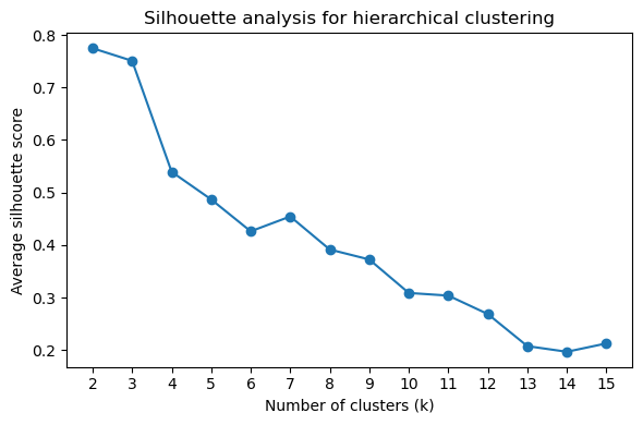
Silhouette and elbow plots guide the choice of cluster number k:
[43]:
# Silhouette score plot (higher = better cluster separation)
pr.pl.hclustv_silhouette(adata, verbose=False)
[44]:
# Elbow plot (look for the "elbow" where inertia decrease slows)
pr.pl.hclustv_elbow(adata, verbose=False)
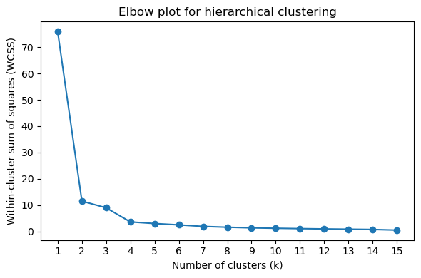
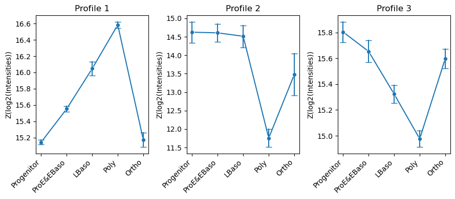
Cluster assignment at k = 3 and mean expression profiles per cluster:
[45]:
# Assign proteins to k=3 clusters and compute cluster profiles
pr.tl.hclustv_cluster_ann(adata, k=3, verbose=False)
pr.tl.hclustv_profiles(adata, verbose=False)
[46]:
# Visualize cluster profiles: mean ± std intensity across cell types for each cluster
pr.pl.hclustv_profile_intensities(
    adata,
    group_by='cell_type',
    order=adata.uns['diff_order'],
    ylabel='Z(log2(Intensities))',
    verbose=False,
    n_cols=3,
    figsize=(9, 4),
    )
Summary
This notebook reproduced key aspects of the protein-level analysis from Karayel et al. (2020) using ProteoPy:
Data quality: High intra-stage reproducibility (Pearson r > 0.95) and ~7,500 quantified protein groups per stage, consistent with the ~7,400 reported in the original study (Figures 1C–D).
Stage separation: PCA resolves the five differentiation stages along the first two principal components, confirming that the dominant source of variation is biological differentiation (Figure 2A).
Differential abundance: One-vs-rest testing identifies hundreds of stage-specific proteins, with the most pronounced changes at the progenitor-to-ProE/EBaso and Poly-to-Ortho transitions, consistent with Figure 2C–D.
Expression profiles: Hierarchical clustering of differentially abundant proteins recovers distinct temporal co-expression patterns across the differentiation trajectory (Figure 2B).